How Many Disposals Do You Need to Get the Umpires' Attention?
/Today we’ll be doing the same, but for umpires’ Brownlow Votes.
UMPIRES’ VOTES AND PLAYER METRICS
As we did for Coaches’ Votes, we’ll treat Brownlow Votes as continuous and then build random forests on samples balanced such that they have the same number of observations for 0 votes, 1 vote, 2 votes, and 3 votes. For one model we’ll have 2,000 of each level, and for the other 5,000.
In the table at right we look at the variable importance from these two new models compared to what we had for the ordinal forest from an earlier blog. Here too we’ve used the permutation metric rather than the Gini impurity metric for the reasons stated in the previous blog.
Once again we find broad similarity between the ranking of the various metrics, especially between those of the models we’ve built especially for this blog. Across the 31 metrics, the maximum ranking difference is just 4 spots and the average only 1.2 spots, due partly to the 11 metrics that have identical rankings in both models.
The largest differences between the rankings of relatively important metrics for the ordinal forest model and these most recent models are for Effective Disposals (from 3rd to 8th), for Team Result (from 11th to 3rd or 4th), and, arguably, for Score Involvements (from 8th to 4th or 2nd).
These differences could be attributable to treating Brownlow Votes as continuous rather than ordinal, or - and more likely, I’d suggest - to working with a balanced rather than a decidedly imbalanced sample. It might well be, for example, that Team Result is very important for separating 1 vote results from 0 votes, but the overwhelming majority of 0 vote results in the imbalanced sample masks this.
In any case, the similarity in the importance rankings for our two new models again gives us license to use the model with the smaller sample size for the remainder of the analysis.
BACK TO THE ICEBOX
Both the Coaches’ Votes model and the latest Brownlow model rank Disposals as the most important metric. Below, on the left, we have the ICE plot for the Brownlow model, while on the right we have the ICE plot for the Coaches’ model from the previous blog.
ICE PLOT FOR THE BROWNLOW MODEL
ICE PLOT FOR THE COACHES’ MODEL
The overall shapes of the conditional expectation lines - those in yellow - are remarkably similar and has little impact on the expected Brownlow or Coaches’ Vote figure until a player gets to about 25 disposals. After that there is a near linear increase in the expectation until we get to about 38 disposals.
In this sense we can conclude that, not ony are umpires and coaches most influenced by Disposal counts in their voting, but that they are similarly affected by counts around the same levels.
The second-most important variable according to both the ordinal model and the ranger model built on 2,000 samples of each level is Goals, and the plots for that metric appears below.
ICE PLOT FOR THE BROWNLOW MODEL
ICE PLOT FOR THE COACHES’ MODEL
Here we see curvilinear relationships between expected votes and Goals from 0 to about 5 goals, but with Brownlow votes tending to increase more rapidly than Coaches’ votes with additional goals. Both are flat for 6 goals and higher.
The third-most important metric for the old and the new model is the Team Result, the plots for which appear below.

ICE PLOT FOR THE BROWNLOW MODEL
ICE PLOT FOR THE COACHES’ MODEL
The shape of the two relationships are remarkably similar, being fairly flat for losses of up to about 50 points and then showing progessive increases in expected votes up to rough maximum at around the level of a draw.
The gallery below contains the plots for the Brownlow model for the metrics ranked 4th to 10th in terms of importance (which, as it happens, are identical to those for the Coaches’ Votes model, and in the same order).


The broad highlights are:
Score Involvements: roughly flat for fewer than 4 then a gentle increase from 4 to about 9 or 10. Flat thereafter. Only a small range from lowest expected Brownlow Votes to highest. Overall, also very similar to the results for Coaches’ Votes.
Contested Possessions: flat for fewer than 4 then a gentle increase from 4 to about 22. Flat thereafter. Smallish range from lowest expected Brownlow Votes to highest. Some small differences between this and Coaches’ Votes for the 16 to 22 Contested Possessions range.
Kicks: roughly flat for fewer than 8 then a gentle increase from 8 to about 20. Flat thereafter. Smallish range from lowest expected Brownlow Votes to highest. Overall, also very similar to the results for Coaches’ Votes.
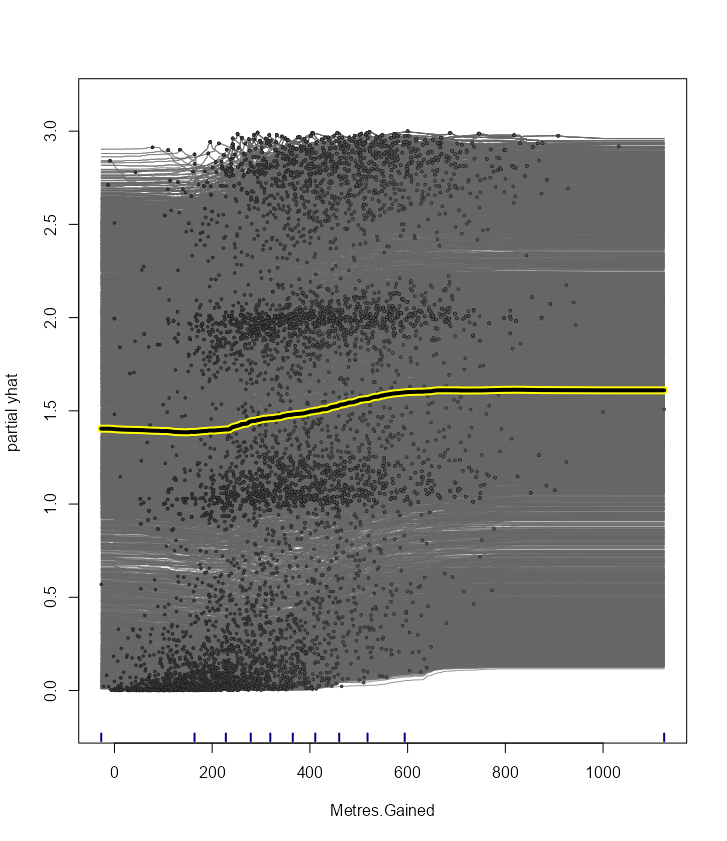
Metres Gained: roughly flat for less than 200m then a gentle increase from 200m to about 500m Flat thereafter. Smallish range from lowest expected Brownlow Votes to highest. Some small differences between this and Coaches’ Votes for the 500m to 700m range.
Effective Disposals: flat for fewer than 8 then a gentle increase from 8 to about 28. Flat thereafter. Very small range from lowest expected Brownlow Votes to highest. Some small differences between this and Coaches’ Votes for the 8 to 12 and 26 to 30 Effective Disposals ranges.
Clearances: gently rises from 1 to 6 clearances. Flat thereafter. Very, very small range from lowest expected Brownlow Votes to highest. Some small differences between this and Coaches’ Votes for the 1 to 5 Clearance range.
Uncontested Possessions: pretty much flat across the entire range of Uncontested Possession counts, as was the case for the Coaches’ Votes model.
So, again, by the time we’ve reached just the 10th-most important variable, the practical importance seems to be close to zero.
And. as we did when looking at Coaches’ Votes, we get an even flatter curve if we plot the results for Goal Assists.
ICE PLOT FOR THE BROWNLOW MODEL
ICE PLOT FOR THE COACHES’ MODEL
SUMMARY AND CONCLUSION
Overall, when we work with balanced samples, we see remarkably similar voting responses to player metrics from umpires and coaches, not just in terms of the relative importance of different metrics (which we’d already noted in this earlier blog), but also in terms of the shapes of the relationships between those metrics and the expected voting values.
That, of course, makes it all the more interesting when coaches’ and umpires’ votes diverge, which is something we’ll look at the next blog.